
Discrete vs Continuous Data
Understanding discrete and continuous data will help you choose the right analysis and visualization methods.

Alex is a tech writer with a background in information security, identity management, and SaaS.
Numerical data can be either continuous or discrete. These data classifications imply using different analytical approaches which determine if your data interpretation is sound. In this guide, we’ll explain the difference between the two data types and explain the most commonly used tools for analyzing and plotting continuous and discrete data.
What is the difference between continuous and discrete data?
Understanding how we use dimensions and measures helps us understand the difference. Most charts in business look something like this:
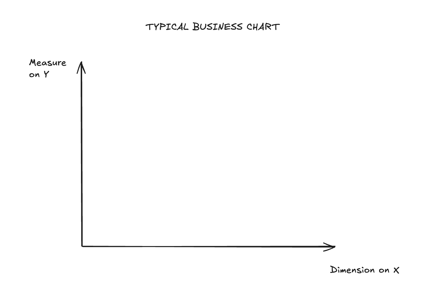
The X axis typically represents time or is categorical. Time has infinite granularity, and thus the dimension is continuous. However, as soon as you aggregate time (e.g., into days), the axis becomes discrete. Categories, on the other hand, don’t have infinite granularity in the first place, so the dimension is discrete from the start.
The Y axis is usually a count or some other kind of aggregation (sum, average, etc.). If it’s a count, it’s a discrete measure, but most other aggregates lead to a continuous Y axis.
So:
Continuous data is measured on a scale that has infinite granularity most of the time. Examples of continuous data are:
- Time between purchases (can be as granular as it gets, weeks or hours)
- Revenue ($, represents a precise monetary value)
Discrete data has a limited set of allowed values and is counted in distinct increments. Some examples of discrete data are:
- Monthly active users (sampled over a rolling 30-day window)
- Number of items per basket (counted per each basket)
Let’s get more practical.
How to Analyze Continuous Data
Many techniques apply to continuous data. The ones you will likely deal with frequently are correlation, distribution, and time series data analysis.
Correlations - Scatter Chart
Correlations help answer questions like:
- Which products are frequently purchased together?
- How do various demographic factors affect purchasing patterns?
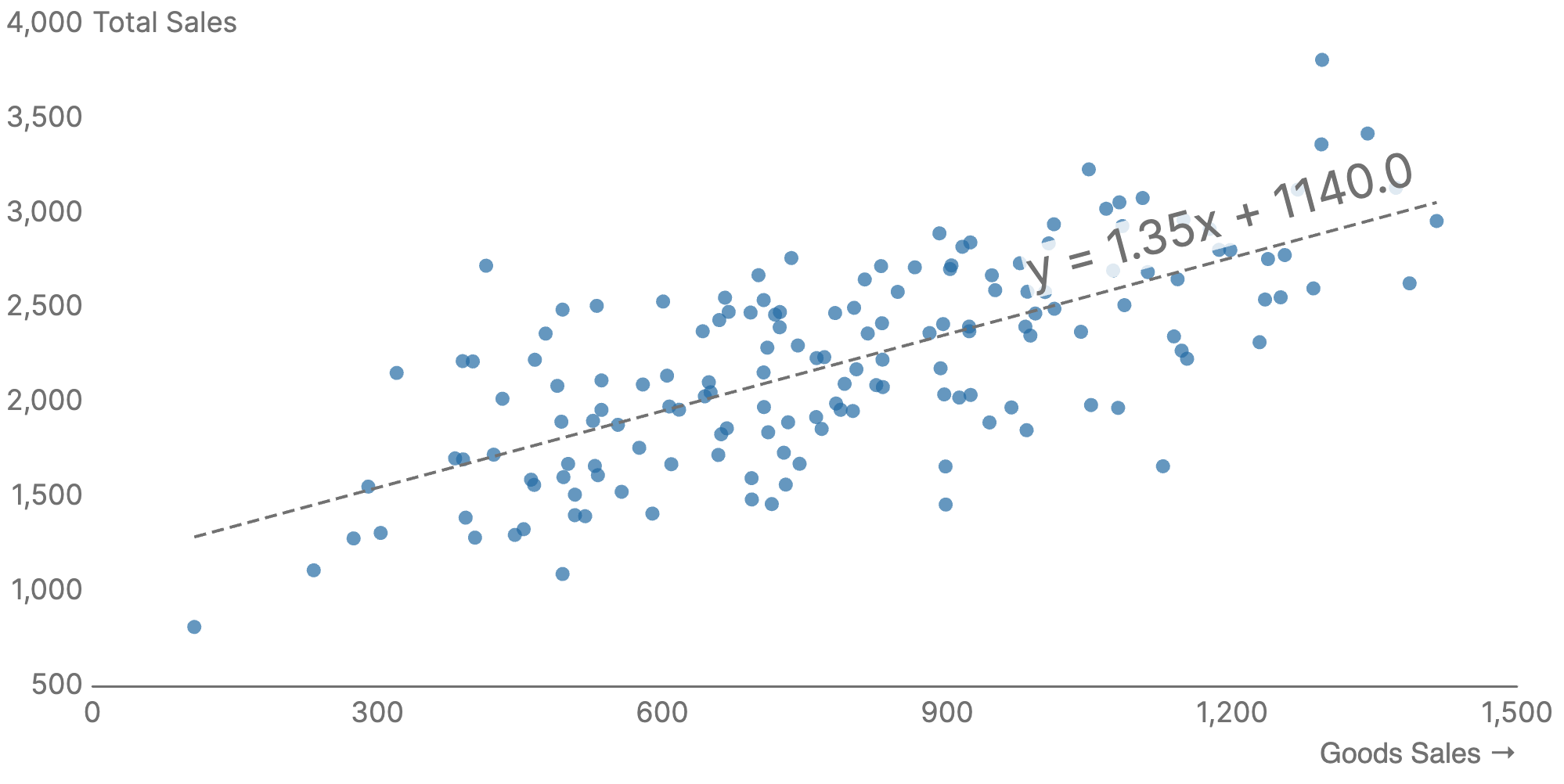
Correlation measures the strength and direction of the relationship between two variables. The analysis will show whether a pair of variables move together positively, negatively, or have little to no linear relationship.
Correlations are often analyzed with a scatter chart—a type of graph that displays values as individual points plotted along two continuous numerical axes (X and Y). On the below chart, it plots the sales of one category against the sales of all categories to see if sales in that category are good predictor of overall spending.
Use scatter charts if you need to:
- Explore relationships between two continuous numeric variables
- Identify patterns, clusters, or outliers
- Visualize cause-and-effect relationships
Distribution - Box Plot
Distribution analysis helps answer questions like:
- What are the slow-moving and fast-moving goods?
- How do sales distribute across categories?
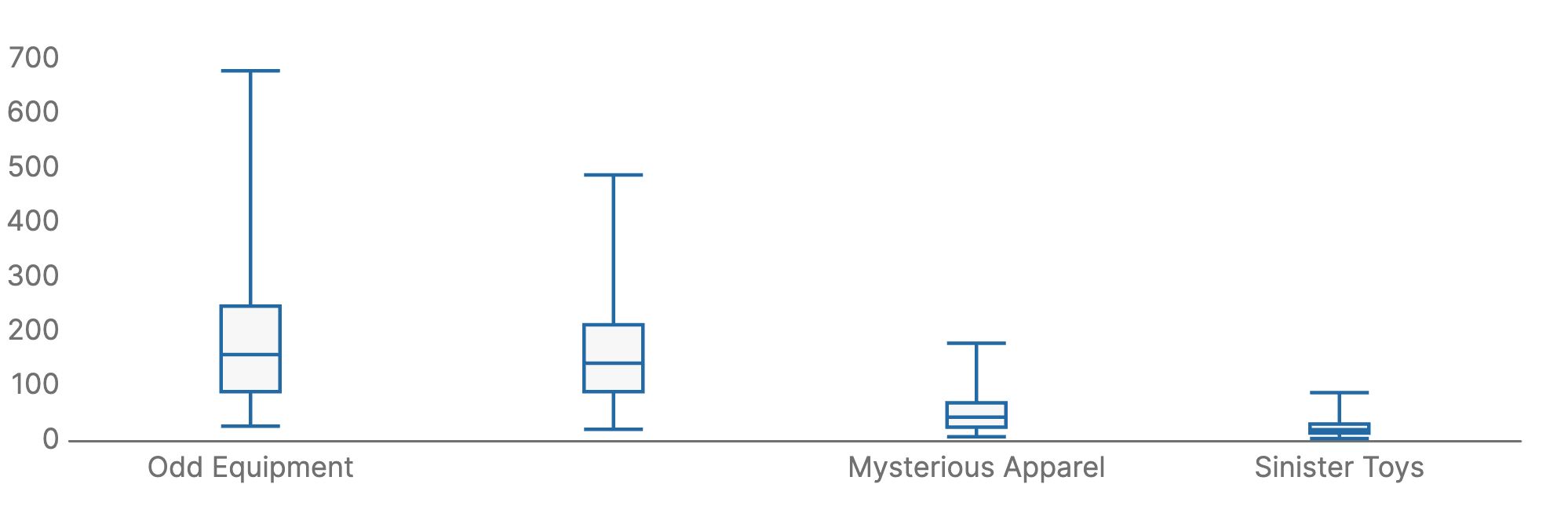
Distribution analysis examines how data points are spread across different values. This helps reveal patterns of frequency and variation.
A common way to analyze the distribution of values is with a box plot that displays the distribution, variability, and outliers of a dataset. Box plots don’t display individual data points. Instead, they show aggregate values—statistical summaries from the original data points. The below example illustrates the distribution of sales over several categories:
Use box plots if you need to:
- Understand data distribution and spread
- Identify outliers in a dataset
- Comparing multiple datasets side by side
- Check for symmetry or skewness in a dataset
Time Series - Line Chart
Time series data analysis helps answer questions like:
- What are the seasonal bestsellers year over year?
- What is the long-term trend for the customer acquisition cost?
Time series data analysis allows you to see how values move over time, and predict future values. Trends and forecasts are typically plotted with either line charts or area charts.
The line chart is a type of graph that represents data points connected by lines. In this case, the chart displays the volumes of sales per day for one year.
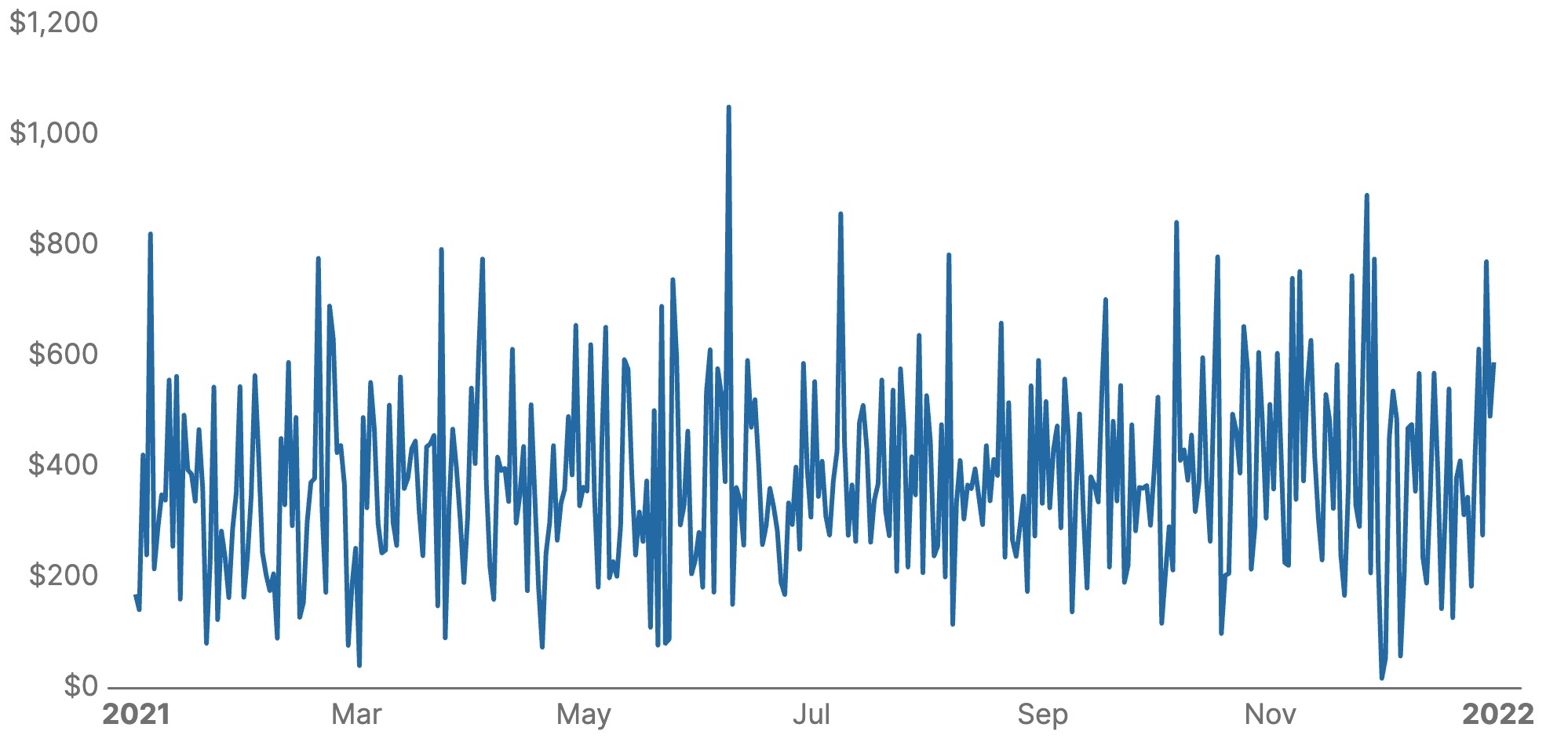
Use line charts if you need to:
- Track trends over time (e.g., sales, website traffic)
- Compare multiple categories over time
- Identify seasonal patterns and fluctuations
- Analyze the rate of change in data
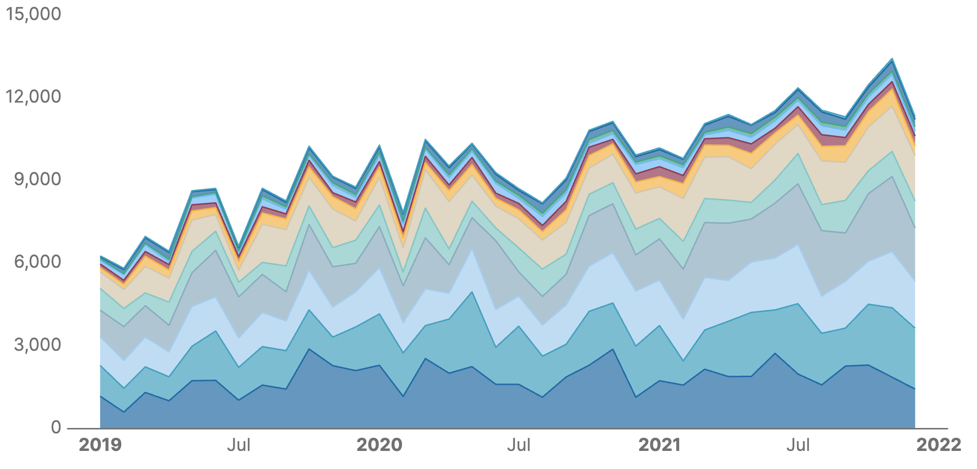
Time Series - Area Chart
The area charts are a variation of a line chart where the area beneath the line is shaded to visualize cumulative values and emphasize volume or magnitude changes. In this case, we plot sales of various items over three years to see overall growth in sales year over year for most items with seasonal dips around January and July/August:
Use area charts if you need to:
- Track trends over time while emphasizing volume
- Display cumulative totals to show dynamics
- Visualize proportions in changing datasets
How to Analyze Discrete Data
Frequency Distribution - Bar Chart
Understanding frequency distribution is one of the most common goals for discrete data. It helps answer questions like:
- How do you segment customers based on their purchase frequency (e.g., daily, weekly, or monthly)?
- How often do customers buy certain items?
Frequency distribution analysis organizes data into categories or intervals to show how often each value occurs. It is often plotted with bar charts that display data divided into distinct categories, such as product types or customer segments (e.g., age groups). Here, we plot sales in various categories over a given time period:
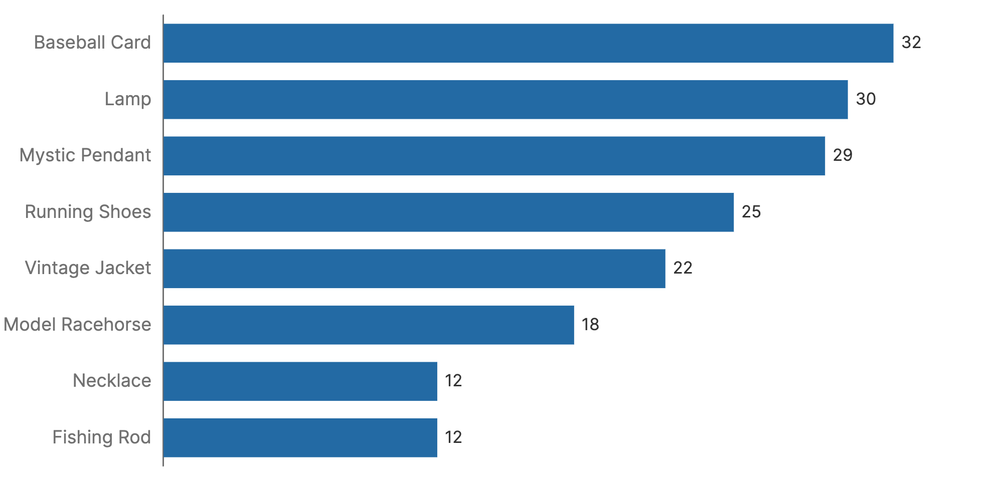
Use bar charts if you need to:
- Compare values across categories, such as revenue by product
- Show rankings, such as best-selling products in a category
- Display discrete data with distinct groups, such as sales by region
- Handle large numbers of categories clearly
Correlation - Heatmap
Correlation analysis applies to discrete data as well. You can plot the results of the analysis with a heatmap chart—a 2D matrix with color coding. In heatmaps, lighter/paler colors are for pairs with weaker correlation, while darker, more saturated colors are for pairs with stronger correlation.
The below example plots a correlation between lead generation channels and actual sales. As you can see, the chart suggest a stronger correlation between PPC campaigns and sales throughout the year (the same goes for organic search), a notable seasonality for Facebook ads, and a very weak correlation between coupons and sales.
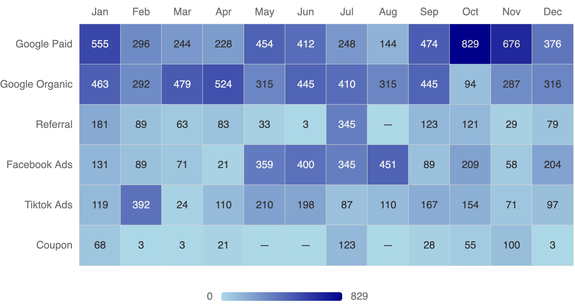
Use heatmaps if you need to:
- Identify correlations and relationships
- Highlight density and intensity, such as sales or user activity
- Track geospatial trends, such as weather or population density
- Examine time-based data patterns, e.g., hourly website visits
Start Analyzing Data with Evidence
All the charts in this article were created with Evidence, a tool for building charts using Markdown and SQL.
